Batch picking, wave picking, zone picking: how to build compact missions to reduce your travel distances

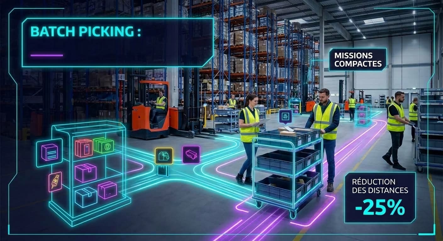
In short:

• Batch picking, wave picking, and zone picking are three order grouping strategies with distinct logics.
• Traditional WMS group by approximate distances: missions remain broad, aisles are unnecessarily traversed.
• Mission compactness is measured by: inter-pick distance, fill rate, aisles traveled.
• A 3D digital twin calculates actual distances and enables geographically coherent batching.
• Measured gains: up to -25% in distances, average 20% improvement in mission building.

Batch, wave, zone picking: what are we talking about?

Three methods, three order grouping logics.

Batch picking

• A picker collects items belonging to several orders in a single run.
• Items are sorted at the end of the run (or en route using multi-order bins).
• Objective: reduce the number of passes over the same locations.

Wave picking

• Orders are released in waves at defined times (carrier departure time, customer priority, shipping window).
• Each wave can combine batch and zone picking.
• Objective: synchronize picking with downstream operational constraints.

Zone picking

• The warehouse is divided into geographic zones; each picker works exclusively in their zone.
• Items from the same order can be picked in parallel in several zones, then consolidated.
• Objective: specialize operators and limit their movements to a reduced area.

In summary:

Batch picking

• Principle: Grouping orders by item or location similarity.
• Typical use case: E-commerce, short orders, high volume of common lines.

Wave picking

• Principle: Grouping by time or operational processing window.
• Typical use case: Multi-carrier warehouses, strong shipping constraints.

Zone picking

• Principle: Grouping by physical warehouse zone.
• Typical use case: Large warehouses, heterogeneous products, temperature-controlled zones.

These three methods are not mutually exclusive: the most efficient mission building combines them according to actual flows.

Why traditional WMS group orders poorly

Two structural limitations explain why batching remains suboptimal in most WMS.

Limitation 1 - Distance accuracy

• WMS calculate distances using simplified 2D coordinates: no levels, no real traffic directions, no physical crossings.
• The distance between two locations is approximated—often as the crow flies or by theoretical aisle—without reflecting the actual path traveled.
• Result: order grouping is geographically incoherent. Two locations considered close by the WMS may be far apart in physical reality.
• Generated missions are broad: the picker crosses aisles without picking, the rate of common picks remains low.

Limitation 2 - Inability to optimize continuously

• The WMS distributes orders as they come in: as soon as an order enters, it is assigned according to the rules set at that moment.
• It does not reconsider supports and orders already in progress or pending.
• It does not recalculate the optimal grouping as new orders arrive.
• Result: compactness opportunities are missed with each wave. An incoming order that could have densified an ongoing mission is assigned elsewhere by default.

Permanent recalculation: the strength of Find & Order

This section directly addresses Limitation 2: the inability of WMS to optimize continuously.

The principle

• Find & Order maintains a global and permanent view of all orders and supports not yet assigned.
• With each new incoming order, the algorithm re-evaluates missions being built to maximize overall compactness.
• This is not a fixed configuration—it's a continuous optimization, recalculated at every event.

What this changes in practice

• Fewer missions open simultaneously: incoming orders densify existing missions rather than opening new ones.
• Higher rate of common picks : locations shared between multiple orders are systematically leveraged.
• Better use of supports: each cart or bin is filled to its optimal capacity before being launched.
• Compactness opportunities are no longer missed between waves—they are captured in real time.

3D digital twin + SMB/MTM method + proprietary algorithms

This section addresses Limitation 1—distance accuracy—and goes further. Three combined layers make permanent recalculation truly effective.

Layer 1 - The 3D digital twin

• Models the warehouse with its real coordinates: aisles, levels, locations, traffic directions, access zones.
• Enables calculation of actual distances between two locations—not 2D approximations.
• Each location is positioned in the exact physical space of the warehouse, including crossings and traffic constraints.

Layer 2 - The SMB method (Methods-Time Measurement / MTM)

• Integrates actual travel times: walking speed, pick time, drop time, handling.
• Enables calculation not just of distances, but of mission times.
• Result: missions are balanced in real time by time, not by number of lines—a much more accurate indicator of operator workload.

Layer 3 - Proprietary flow algorithms

• Combine the 3D digital twin and SMB/MTM method to build optimal missions.
• Simultaneously consider spatial compactness, actual times, and operational constraints (support capacity, FIFO/FEFO, temperature zones).
• Produce order groupings that maximize pick density within the smallest possible area.

Why these three layers are inseparable

• Without distance accuracy (3D twin), continuous optimization produces compact missions on paper, incoherent in the real warehouse.
• Without time calculation (SMB/MTM), missions are balanced by lines but not by actual workload—some pickers finish early, others are overloaded.
• Without flow algorithms, the first two layers remain raw data without operational translation.

WMS alone vs Find & Order: summary

Distance accuracy

• WMS alone: Approximate (calculation based on simplified 2D coordinates).
• Find & Order: Actual (3D modeling including aisles, levels, and traffic directions).

Continuous optimization

• WMS alone: Static (order distribution as they come in).
• Find & Order: Permanent recalculation (re-evaluation with each incoming order).

Mission time calculation

• WMS alone: Absent (simple balancing by number of lines).
• Find & Order: Integrated SMB/MTM method (balancing based on actual times).

Mission compactness

• WMS alone: Variable and often low.
• Find & Order: Optimized (reduced area and maximized rate of common picks).

Dependence on manual configuration

• WMS alone: High (requires regular adjustments).
• Find & Order: Low (automatic recalculation adjusted to actual flows).

Operational constraints: what batching must integrate

Optimal geographic grouping is not enough—mission building must integrate real operational constraints.

Multi-SKUs

• Product compatibility: avoid grouping SKUs that could be confused (similar packaging, close sizes).
• Pick sequencing: the pick order within the mission must limit sorting errors.
• Rate of common picks: maximize locations shared between multiple orders in the same mission.

Weight and volume

• Support capacity (cart, bin, pallet): order grouping must not exceed the maximum allowable load.
• Load balance: distribute weight to avoid imbalances on the picking support.
• Total mission volume: anticipate available space for large items.

Temperature-controlled zones

• Limited exposure time: chilled or frozen products must be picked last or in dedicated missions.
• Grouping by thermal zone: build separate missions for cold zones to limit cold chain breaks.

Other constraints to integrate

• FIFO / FEFO: respect the release order by receipt date or expiration date.
• Hazardous products: mandatory segregation, dedicated missions according to applicable regulations.
• Secured zones: restricted access to certain locations (high-value products, quality control area).

KPIs to measure batching impact

Six KPIs to manage mission building performance.

1. Number of missions generated

• Definition: total number of missions created to process a given order volume.
• What an improvement means: fewer missions = less empty travel, less handling time, better use of pickers.

2. Mission fill rate

• Definition: support capacity used (bins, cart, pallet) relative to its maximum capacity.
• What an improvement means: each trip carries more goods—the number of passes over locations decreases.

3. Number of trips per mission

• Definition: number of route segments made between the start and end of a mission.
• What an improvement means: fewer trips = reduced picking time, less operator fatigue.

4. Rate of common picks

• Definition: share of picks shared between multiple orders in the same mission (same location visited for several orders).
• What an improvement means: the picker picks several orders in a single pass—the location is visited only once for multiple orders.

5. Number of aisles traveled per mission

• Definition: number of distinct aisles crossed to complete a mission.
• What an improvement means: a compact mission stays within a reduced area—fewer aisles = less inter-pick distance.

6. Inter-pick distance

• Definition: average distance between two consecutive picks within the same mission.
• What an improvement means: direct indicator of the geographic compactness of batching—its reduction validates that order grouping is spatially coherent.

Concrete results: what optimized batching changes

Measured gains in mission building

• Up to -25% in distances traveled by pickers.
• Average 20% gain in mission building productivity.
• Reduction in the number of missions generated for the same order volume.

Leverage effect with other modules

• Building compact missions: average 20% gain
• Optimized picking paths: average 10% gain (up to -20% depending on traffic constraints)
• Slotting: average 25% gain (up to -30% on picking distances)
• These levers are cumulative: each optimization applies to a flow already improved by the previous ones.

What this means in practice

• Fewer kilometers traveled per picker and per shift.
• Increased picks per hour without adding resources.
• Reduced operator fatigue in high-movement roles.

-> Estimate your potential gains with the Find & Order gain calculator.

FAQ

What is the difference between batch picking and wave picking?

The batch picking groups orders based on the similarity of their locations: a picker collects several orders in a single run to avoid returning to the same place multiple times.

The wave picking groups orders according to a time or operational window (carrier departure time, customer priority): orders are released in waves at defined times. The two methods are complementary—a wave can contain several batches, each created based on a geographic criterion.

Is it necessary to change WMS to optimize task creation?

No. The optimization layer integrates on top of the existing WMS, without replacement or overhaul. The WMS continues to manage inventory, receiving, and shipping. The optimization of task creation, picking paths, and slotting is handled by a dedicated software layer that uses WMS data and returns optimized tasks to it. Integration is done via API or standard connector.

How can I measure the ROI of batching in my warehouse?

Three indicators are enough for an initial ROI calculation:

• Inter-pick distance before / after : direct measurement of task compactness.
• Number of tasks generated for the same order volume: fewer tasks = less handling time and fewer empty trips.
• Picks per hour per picker : overall productivity indicator, directly impacted by reduced travel.

A full ROI calculation also includes the hourly cost of pickers, the order volume processed per shift, and gains from other levers (picking paths, slotting). The gains calculator allows you to estimate these gains based on your actual data.